Project 3 : House Prices Prediction

House prices can vary by house and alot of different factors can influence the price of a house. I will try to use regression to predict house prices from a dataset depending on various factors like total squarefeet and the amount of bedrooms and much more.
The Data
The data set is from Kaggle and contains house prices and features from Ames, Iowa
the data set was created by Kaggle for a competition.
Linear Regression is a way to model the estimate of relationships between a dependent variable and with one or multiple independent variables. For linear regression we use the following formula to help us plot the data.
y = mx+b
y = dependent variable
x = independent variable
m = predicted slope
b = predicted intercept
What is Linear Regression ?
Data Understanding

I know its hard to see but according to the heat map we have some really important correlations and some that are not so important. For categories that are most correlated with price they are Quality of the Overall House and the Garage Living Area. It also gave me an insight on categories to drop like Month sold and Year sold.
Pre-Processing
The data overall does not have any nulls, however there is alot of categories that are listed which I believe do not affect the price of a house and will not help predict the cost of a house.
I end up dropping MonthSold, YearSold, Street, Alley and YearBuilt.

Modeling
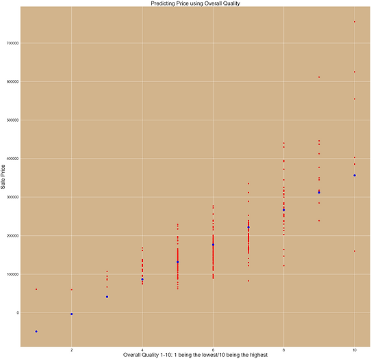
I used Overall Quality as feature to use to predict house sale prices. Since Overall Quality had the highest correlation to house sale prices at 0.79.
Experiment 1 : Evaluation
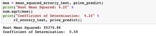
Overall, the model was pretty accurate over 0.50 for the Coefficient of Determination which was 0.59. I think using Overall Quality as predictor is very important but I think we should add another feature to help increase the Coefficient of Determination.
Experiment 2: Evaluation


The graph shows predicting houses prices based upon the Garage Living Area which is the total area in the garage in square feet. This feature also had second best correlation to house prices. The graph shows that the bigger the area in the garage, more than likely the price of the house is greater as well. The correlation between houses prices and garage living area looked very strong.
Adding another feature helped our model increase its acccuracy and it shows, the Coefficent of Determination went from 0.59 to 0.62. Not the biggest jump but still helps our model be more accurate in predicting house prices.
Experiment 3: Evaluation

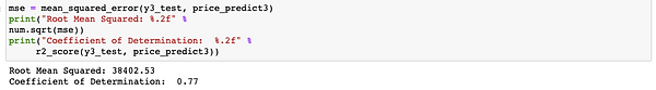
The graph shows predicting house prices with the feature Garage Cars, which is the amount of cars a house can fit in the garage. The Garage Cars feature had the 3rd highest correlation to Sale Price which is why it was chosen in the third experiment. The graph shows using the feature is very accurate because the correlation is very high.
Looking at tests for the final experiment the accuracy for our predictor model went up. Looking at the Coefficent of Determination it went from 0.62 to 0.77 with now all three features being used to predict house prices.
Impact
The data shows that Quality was the most important feature for resident in Ames, Iowa when looking for a house. After that the features that followed suprised me, they were mostly to do with the garage. This suprised me because most people I know talk about how big they want their kitchen or bedroom, but the residents of Ames beg to differ. Now of course in Iowa the winters there are very harsh and keeping vehicles and other items inside is important. This also shows that feature importance probably changes depending on environment and other key factors, meaning I would not be able to use this predictor model for house prices in Miami.
Conclusion
This project helped me understand why linear regression was very useful in being used to predict and find associations between two variables. I also learned that the more features I used the better predicitions I could get with the model. In terms of this model I believe if added the next highest correlated features (according to the heatmap) to the model, the coefficient of determination would have been over 0.90, making the model even more accurate.